Split Plot — splot • splot

A plotting function aimed at automating some common visualization tasks in order to ease data exploration.

Usage

splot(y, data = NULL, su = NULL, type = "", split = "median",
  levels = list(), sort = NULL, error = "standard",
  error.color = "#585858", error.lwd = 2, lim = 9, lines = TRUE, ...,
  colors = "pastel", colorby = NULL, colorby.leg = TRUE,
  color.lock = FALSE, color.offset = 1.1, color.summary = "mean",
  opacity = 1, dark = getOption("splot.dark", FALSE), x = NULL,
  by = NULL, between = NULL, cov = NULL, line.type = "l",
  mv.scale = "none", mv.as.x = FALSE, save = FALSE, format = cairo_pdf,
  dims = dev.size(), file.name = "splot", myl = NULL, mxl = NULL,
  autori = TRUE, xlas = 0, ylas = 1, xaxis = TRUE, yaxis = TRUE,
  breaks = "sturges", density.fill = TRUE, density.opacity = 0.4,
  density.args = list(), leg = "outside", lpos = "auto", lvn = TRUE,
  leg.title = TRUE, leg.args = list(), title = TRUE, labx = TRUE,
  laby = TRUE, lty = TRUE, lwd = 2, sub = TRUE, ndisp = TRUE,
  note = TRUE, font = c(title = 2, sud = 1, leg = 1, leg.title = 2, note =
  3), cex = c(title = 1.5, sud = 0.9, leg = 0.9, note = 0.7, points = 1),
  sud = TRUE, labels = TRUE, labels.filter = "_", labels.trim = 20,
  points = TRUE, points.first = TRUE, byx = TRUE, drop = c(x = TRUE, by
  = TRUE, bet = TRUE), prat = c(1, 1), check.height = TRUE,
  model = FALSE, options = NULL, add = NULL)

Arguments

y: a formula (see note), or the primary variable(s) to be shown on the y axis (unless x is not specified). When not a formula, this can be one or more variables as objects, or names in data.
data: a data.frame to pull variables from. If variables aren't found in data, they will be looked for in the environment.
su: a subset to all variables, applied after they are all retrieved from data or the environment.
type: determines the type of plot to make, between "bar", "line", "density", or "scatter". If "density", x is ignored. Anything including the first letter of each is accepted (e.g., type='l').
split: how to split any continuous variables (those with more than lim levels as factors). Default is "median", with "mean", "standard deviation", "quantile", or numbers as options. If numbers, the variable is either cut at each value in a vector, or broken into roughly equal chunks. Entering an integer (e.g., split = 3L) that is greater than 1 will force splitting into segments. Otherwise variables will be split by value if you enter a single value for split and there are at least two data less than or equal to and greater than the split, or if you enter more than 1 value for split. If a numeric split is not compatible with splitting by value or segment, splitting will default to the median.
levels: a list with entries corresponding to variable names, used to rename and/or reorder factor levels. To reorder a factor, enter a vector of either numbers or existing level names in the new order (e.g., levels = list(var = c(3,2,1))). To rename levels of a factor, enter a character vector the same length as the number of levels. To rename and reorder, enter a list, with names as the first entry, and order as the second entry (e.g., levels = list(var = list(c('a','b','c'), c(3,2,1)))). This happens after variables are split, so names and orders should correspond to the new split levels of split variables. For example, if a continuous variable is median split, it now has two levels ('Under Median' and 'Over Median'), which are the levels reordering or renaming would apply to. Multiple variables entered as y can be renamed and sorted with an entry titled 'mv'.
sort: specified the order of character or factor x levels. By default, character or factor x levels are sorted alphabetically. FALSE will prevent this (preserving entered order). TRUE or 'd' will sort by levels of y in decreasing order, and anything else will sort in increasing order.
error: string; sets the type of error bars to show in bar or line plots, or turns them off. If FALSE, no error bars will be shown. Otherwise, the default is "standard error" ('^s'), with "confidence intervals" (anything else) as an option.
error.color: color of the error bars. Default is '#585858'.
error.lwd: line weight of error bars. Default is 2.
lim: numeric; checked against the number of factor levels of each variable. Used to decide which variables should be split, which colors to use, and when to turn off the legend. Default is 9. If set over 20, lim is treated as infinite (set to Inf).
lines: logical or a string specifying the type of lines to be drawn in scatter plots. By default (and whenever cov is not missing, or if lines matches '^li|^lm|^st'), a prediction line is fitted with lm. For (potentially) bendy lines, 'loess' (matching '^loe|^po|^cu') will use loess, and 'spline' ('^sm|^sp|^in') will use smooth.spline. If y is not numeric and has only 2 levels, 'probability' ('^pr|^log') will draw probabilities estimated by a logistic regression (glm(y ~ x, binomial)). 'connected' ('^e|^co|^d') will draw lines connecting all points, and FALSE will not draw any lines.
...: passes additional arguments to par or legend. Arguments before this can be named partially; those after must by fully named.
colors: sets a color theme or manually specifies colors. Default theme is "pastel", with "dark" and "bright" as options; these are passed to splot.color. If set to "grey", or if by has more than 9 levels, a grey scale is calculated using gray. See the col parameter in par for acceptable manual inputs. To set text and axis colors, col sets outside texts (title, sud, labx, laby, and note), col.sub or col.main sets the frame titles, and col.axis sets the axis text and line colors. To set the color of error bars, use error.color. For histograms, a vector of two colors would apply to the density line and bars separately (e.g., for color = c('red','green'), the density line would be red and the histogram bars would be green). See the color.lock and color.offset arguments for more color controls.
colorby: a variable or list of arguments used to set colors and the legend, alternatively to by. If by is not missing, colorby will be reduced to only the unique combinations of by and colorby. For example, if by is a participant ID with multiple observations per participant, and by is a condition ID which is the same for all observations from a given participant, colorby would assign a single color to each participant based on their condition. A list will be treated as a call to splot.color, so arguments can be entered positionally or by name. Data entered directly into splot can be accessed by position name preceded by a period. For example, splot(rnorm(100), colorby=.y) would draw a histogram, with bars colored by the value of y (rnorm(100) in this case).
colorby.leg: logical; if FALSE, a legend for colorby is never drawn. Otherwise, a legend for colorby will be drawn if there is no specified by, or for non-scatter plots (overwriting the usual legend).
color.lock: logical; if FALSE, colors will not be adjusted to offset lines from points or histogram bars.
color.offset: how much points or histogram bars should be offset from the initial color used for lines. Default is 1.1; values greater than 1 lighten, and less than 1 darken.
color.summary: specifies the function used to collapse multiple colors for a single display. Either a string matching one of 'mean' (which uses splot.colormean to average RGB values), 'median' ( which treats codes as ordered, and selects that at the rounded median), or 'mode' (which selects the most common code), or a function which takes color codes in its first argument, and outputs a single color code as a character.
opacity: a number between 0 and 1; sets the opacity of points, lines, and bars. Semi-opaque lines will sometimes not be displayed in the plot window, but will show up when the plot is written to a file.
dark: logical; if TRUE, sets text and axis colors to "white". Defaults to the splot.dark option.
x: secondary variable, to be shown in on the x axis. If not specified, type will be set to 'density'. If x is a factor or vector of characters, or has fewer than lim levels when treated as a factor, type will be set to 'line' unless specified.
by: the 'splitting' variable within each plot, by which the plotted values of x and y will be grouped.
between: a single object or name, or two in a vector (e.g., c(b1, b2)), the levels of which will determine the number of plot windows to be shown at once (the cells in a matrix of plots; levels of the first variable as rows, and levels of the second as columns).
cov: additional variables used for adjustment. Bar and line plots include all cov variables in their regression models (via lm, e.g., lm(y ~ 0 + x + cov1 + cov2)) as covariates. Scatter plots with lines include all cov variables in the regression model to adjust the prediction line (e.g., lm(y ~ x + x^2)). par options col, mfrow, oma, mar, mgp, font.main, cex.main, font.lab, tcl, pch, lwd, and xpd are all set within the function, but will be overwritten if they are included in the call. For example, col sets font colors in this case (as opposed to colors which sets line and point colors). The default is '#303030' for a nice dark grey, but maybe you want to lighten that up: col='#606060'. After arguments have been applied to par, if any have not been used and match a legend argument, these will be applied to legend.
line.type: a character setting the style of line (e.g., with points at joints) to be drawn in line plots. Default is 'b' if error is FALSE, and 'l' otherwise. See the line argument of plot.default for options. line.type='c' can look nice when there aren't a lot of overlapping error bars.
mv.scale: determines whether to center and scale multiple y variables. Does not center or scale by default. Anything other than 'none' will mean center each numeric y variable. Anything matching '^t|z|sc' will also scale.
mv.as.x: logical; if TRUE, variable names are displayed on the x axis, and x is treated as by.
save: logical; if TRUE, an image of the plot is saved to the current working directory.
format: the type of file to save plots as. Default is cairo_pdf; see Devices for options.
dims: a vector of 2 values (c(width, height)) specifying the dimensions of a plot to save in inches or pixels depending on format. Defaults to the dimensions of the plot window.
file.name: a string with the name of the file to be save (excluding the extension, as this is added depending on format).
myl: sets the range of the y axis (ylim of plot or barplot). If not specified, this will be calculated from the data.
mxl: sets the range of the x axis (xlim of plot). If not specified, this will be calculated from the data.
autori: logical; if FALSE, the origin of plotted bars will be set to 0. Otherwise, bars are adjusted such that they extend to the bottom of the y axis.
xlas, ylas: numeric; sets the orientation of the x- and y-axis labels. See par.
xaxis, yaxis: logical; if FALSE, the axis will not be drawn.
breaks: determines the width of histogram bars. See hist.
density.fill: logical; FALSE will turn off polygon fills when they are displayed, TRUE will replace histograms with polygons.
density.opacity: opacity of the density polygons, between 0 and 1.
density.args: list of arguments to be passed to density.
leg: sets the legend inside or outside the plot frames (when a character matching '^i', or a character matching '^o' or a number respectively), or turns it off (when FALSE). When inside, a legend is drawn in each plot frame. When outside, a single legend is drawn either to the right of all plot frames, or within an empty plot frame. By default, this will be determined automatically, tending to set legends outside when there are multiple levels of between. A number will try and set the legend in an empty frame within the grid of plot frames. If there are no empty frames, the legend will just go to the side as if leg='outside'.
lpos: sets the position of the legend within its frame (whether inside or outside of the plot frames) based on keywords (see legend. By default, when the legend is outside, lpos is either 'right' when the legend is in a right-hand column, or 'center' when in an empty plot frame. When the legend is inside and lpos is not specified, the legend will be placed automatically based on the data. Set to 'place' to manually place the legend; clicking the plot frame will set the top left corner of the legend.
lvn: level variable name. Logical: if FALSE, the names of by and between variables will not be shown before their level (e.g., for a sex variable with a "female" level, "sex: female" would become "female" above each plot window).
leg.title: sets the title of the legend (which is the by variable name by default), or turns it off with FALSE.
leg.args: a list passing arguments to the legend call.
title: logical or a character: if FALSE, the main title is turned off. If a character, this will be shown as the main title.
labx, laby: logical or a character: if FALSE, the label on the x axis is turned off. If a character, this will be shown as the axis label.
lty: logical or a vector: if FALSE, lines are always solid. If a vector, changes line type based on each value. Otherwise loops through available line types, see par.
lwd: numeric; sets the weight of lines in line, density, and scatter plots. Default is 2. See par.
sub: affects the small title above each plot showing between levels; text replaces it, and FALSE turns it off.
ndisp: logical; if FALSE, n per level is no longer displayed in the subheadings.
note: logical; if FALSE, the note at the bottom about splits and/or lines or error bars is turned off.
font: named numeric vector: c(title,sud,leg,leg.title,note). Sets the font of the title, su display, legend levels and title, and note. In addition, font.lab sets the x and y label font, font.sub sets the font of the little title in each panel, font.axis sets the axis label font, and font.main sets the between level/n heading font; these are passed to par. See the input section.
cex: named numeric vector: c(title,sud,leg,note,points). Sets the font size of the title, su display, legend, note, and points. In addition, cex.lab sets the x and y label size, cex.sub sets the size of the little title in each panel, cex.axis sets the axis label size, and cex.main sets the between level/n heading size; these are passed to par. See the input section.
sud: affects the heading for subset and covariates/line adjustments (su display); text replaces it, and FALSE turns it off.
labels: logical; if FALSE, sets all settable text surrounding the plot to FALSE (just so you don't have to set all of them if you want a clean frame).
labels.filter: a regular expression string to be replaced in label texts with a blank space. Default is '_', so underscores appearing in the text of labels are replace with blank spaces. Set to FALSE to prevent all filtering.
labels.trim: numeric or logical; the maximum length of label texts (in number of characters). Default is 20, with any longer labels being trimmed. Set to FALSE to prevent any trimming.
points: logical; if FALSE, the points in a scatter plot are no longer drawn.
points.first: logical; if FALSE, points are plotted after lines are drawn in a scatter plot, placing lines behind points. This does not apply to points or lines added in add, as that is always evaluated after the main points and lines are drawn.
byx: logical; if TRUE (default) and by is specified, regressions for bar or line plots compare levels of by for each level of x. This makes for more intuitive error bars when comparing levels of by within a level of x; otherwise, the model is comparing the difference between the first level of x and each of its other levels.
drop: named logical vector: c(x,by,bet). Specifies how levels with no data should be treated. All are TRUE by default, meaning only levels with data will be presented, and the layout of between levels will be minimized. x only applies to bar or line plots. by relates to levels presented in the legend. If bet is FALSE, the layout of between variables will be strict, with levels of between[1] as rows, and levels of between[2] as columns -- if there are no data at an intersection of levels, the corresponding panel will be blank. See the input section.
prat: panel ratio, referring to the ratio between plot frames and the legend frame when the legend is out. A single number will make all panels of equal width. A vector of two numbers will adjust the ratio between plot panels and the legend panel. For example, prat=c(3,1) makes all plot panels a relative width of 3, and the legend frame a relative width of 1.
check.height: logical; if FALSE, the height of the plot frame will not be checked before plotting is attempted. The check tries to avoid later errors, but may prevent plotting when a plot is possible.
model: logical; if TRUE, the summary of an interaction model will be printed. This model won't always align with what is plotted since variables may be treated differently, particularly in the case of interactions.
options: a list with named arguments, useful for setting temporary defaults if you plan on using some of the same options for multiple plots (e.g., opt = list(type = 'bar', colors = 'grey', bg = '#999999'); splot(x ~ y, options = opt)). use quote to include options that are to be evaluated within the function (e.g., opt = list(su = quote(y > 0))).
add: evaluated within the function, so you can refer to the objects that are returned, to variable names (those from an entered data frame or entered as arguments), or entered data by their position, preceded by '.' (e.g., mod = lm(.y~.x)). Useful for adding things like lines to a plot while the parameters are still those set by the function (e.g., add = abline(v = mean(x), xpd = FALSE) for a vertical line at the mean of x).

Value

A list containing data and settings is invisibly returned, which might be useful to check for errors. Each of these objects can also be pulled from within add:

`dat`	a `data.frame` of processed, unsegmented data.
`cdat`	a `list` of `list`s of `data.frame`s of processed, segmented data.
`txt`	a `list` of variable names. used mostly to pull variables from `data` or the environment.
`ptxt`	a `list` of processed variable and level names. Used mostly for labeling.
`seg`	a `list` containing segmentation information (such as levels) for each variable.
`ck`	a `list` of settings.
`lega`	a `list` of arguments that were or would have been passed to `legend`.
`fmod`	an `lm` object if `model` is `TRUE`, and the model succeeded.

Note

x-axis levels text

If the text of x-axis levels (those corresponding to the levels of x) are too long, they are hidden before overlapping. To try and avoid this, by default longer texts are trimmed (dictated by labels.trim), and at some point the orientation of level text is changed (settable with xlas), but you may still see level text missing. To make these visible, you can reduce labels.trim from the default of 20 (or rename the levels of that variable), make the level text vertical (xlas = 3), or expand your plot window if possible.

missing levels, lines, and/or error bars

By default (if drop = TRUE), levels of x with no data are dropped, so you may not see every level of your variable, at all or at a level of by or between. Sometimes error bars cannot be estimated (if, say, there is only one observation at the given level), but lines are still drawn in these cases, so you may sometimes see levels without error bars even when error bars are turned on. Sometimes (particularly when drop['x'] is FALSE), you might see floating error bars with no lines drawn to them, or what appear to be completely empty levels. This happens when there is a missing level of x between two non-missing levels, potentially making an orphaned level (if a non-missing level is surrounded by missing levels). If there are no error bars for this orphaned level, by default nothing will be drawn to indicate it. If you set line.type to 'b' (or any other type with points), a point will be drawn at such error-bar-less, orphaned levels.

unexpected failures

splot tries to clean up after itself in the case of an error, but you may still run into errors that break things before this can happen. If after a failed plot you find that you're unable to make any new plots, or new plots are drawn over old ones, you might try entering dev.off() into the console. If new plots look off (splot's par settings didn't get reset), you may have to close the plot window to reset par (if you're using RStudio, Plots > "Remove Plot..." or "Clear All..."), or restart R.

Input

formulas

When y is a formula (has a ~), other variables will be pulled from it:

y ~ x * by * between[1] * between[2] + cov[1] + cov[2] + cov[n]

If y has multiple variables, by is used to identify the variable (it becomes a factor with variable names as levels), so anything entered as by is treated as between[1], between[1] is moved to between[2], and between[2] is discarded with a message.

named vectors

Named vector arguments like font, cex, and drop can be set with a single value, positionally, or with names. If a single value is entered (e.g., drop = FALSE), this will be applied to each level (i.e., c(x = FALSE, by = FALSE, bet = FALSE)). If more than one value is entered, these will be treated positionally (e.g., cex = c(2, 1.2) would be read as c(title = 2, sud = 1.2, leg = .9, note = .7, points = 1)). If values are named, only named values will be set, with other defaults retained (e.g., cex = c(note = 1.2) would be read as c(title = 1.5, sud = .9, leg = .9, note = 1.2, points = 1)).

Examples

# simulating data
n <- 2000
dat <- data.frame(sapply(c("by", "bet1", "bet2"), function(c) sample(0:1, n, TRUE)))
dat$x <- with(
  dat,
  rnorm(n) + by * -.4 + by * bet1 * -.3 + by * bet2 *
    .3 + bet1 * bet2 * .9 - .8 + rnorm(n, 0, by)
)
dat$y <- with(
  dat,
  x * .2 + by * .3 + bet2 * -.6 + bet1 * bet2 * .8 + x *
    by * bet1 * -.5 + x * by * bet1 * bet2 * -.5
    + rnorm(n, 5) + rnorm(n, -1, .1 * x^2)
)

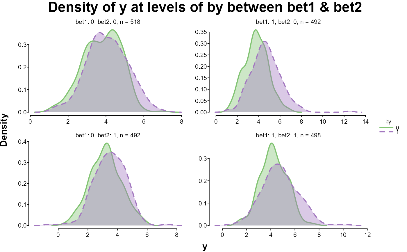
# looking at the distribution of y between bets split by by
splot(y, by = by, between = c(bet1, bet2), data = dat)


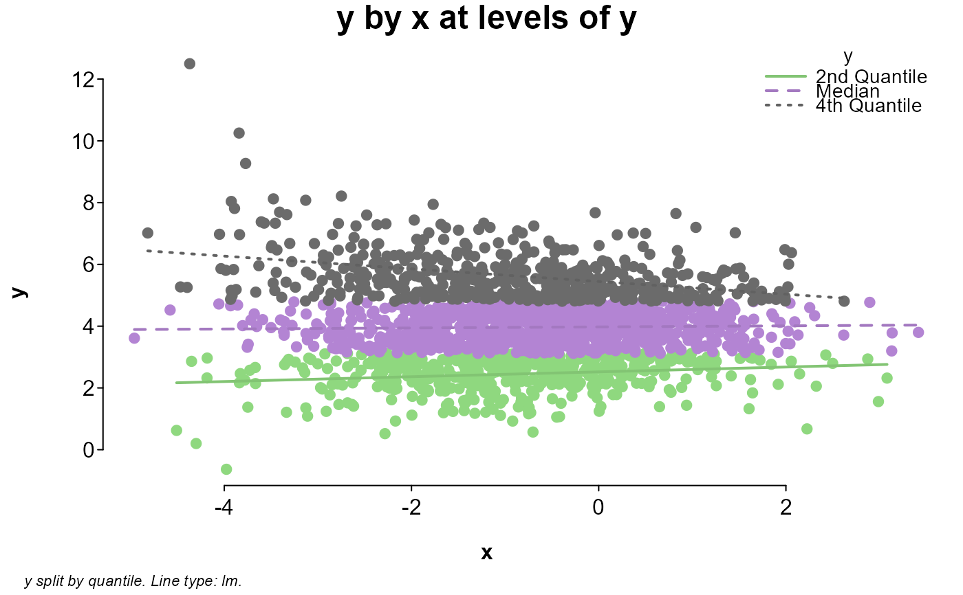
# looking at quantile splits of y in y by x
splot(y ~ x * y, dat, split = "quantile")


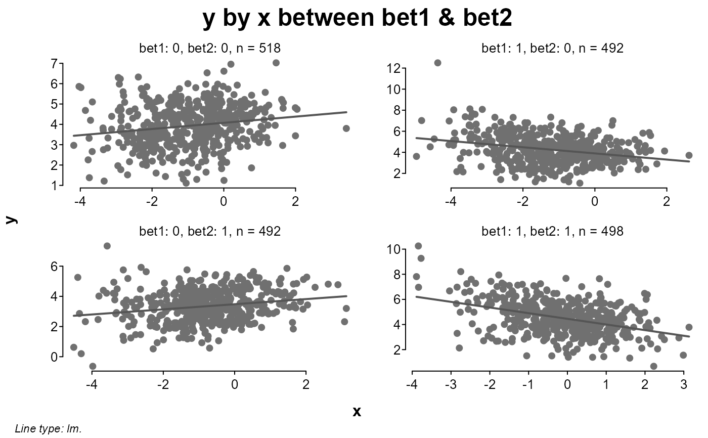
# looking at y by x between bets
splot(y ~ x, dat, between = c(bet1, bet2))


# sequentially adding levels of split
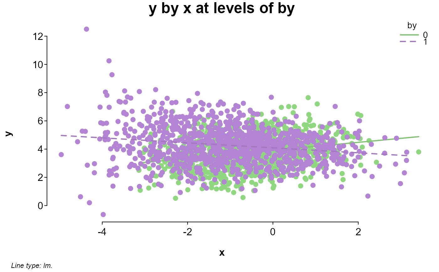
splot(y ~ x * by, dat)

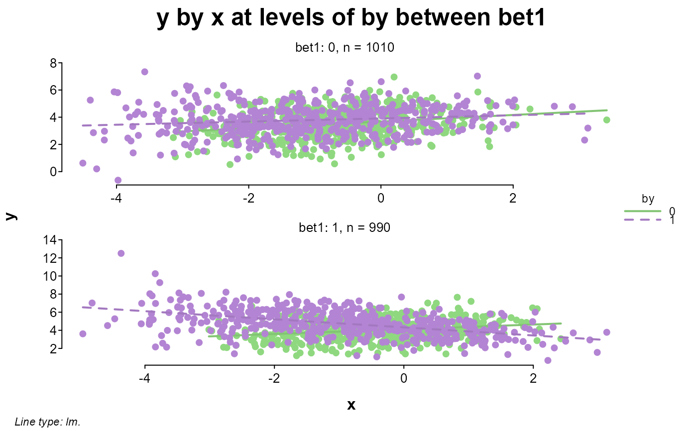
splot(y ~ x * by * bet1, dat)

splot(y ~ x * by * bet1 * bet2, dat)


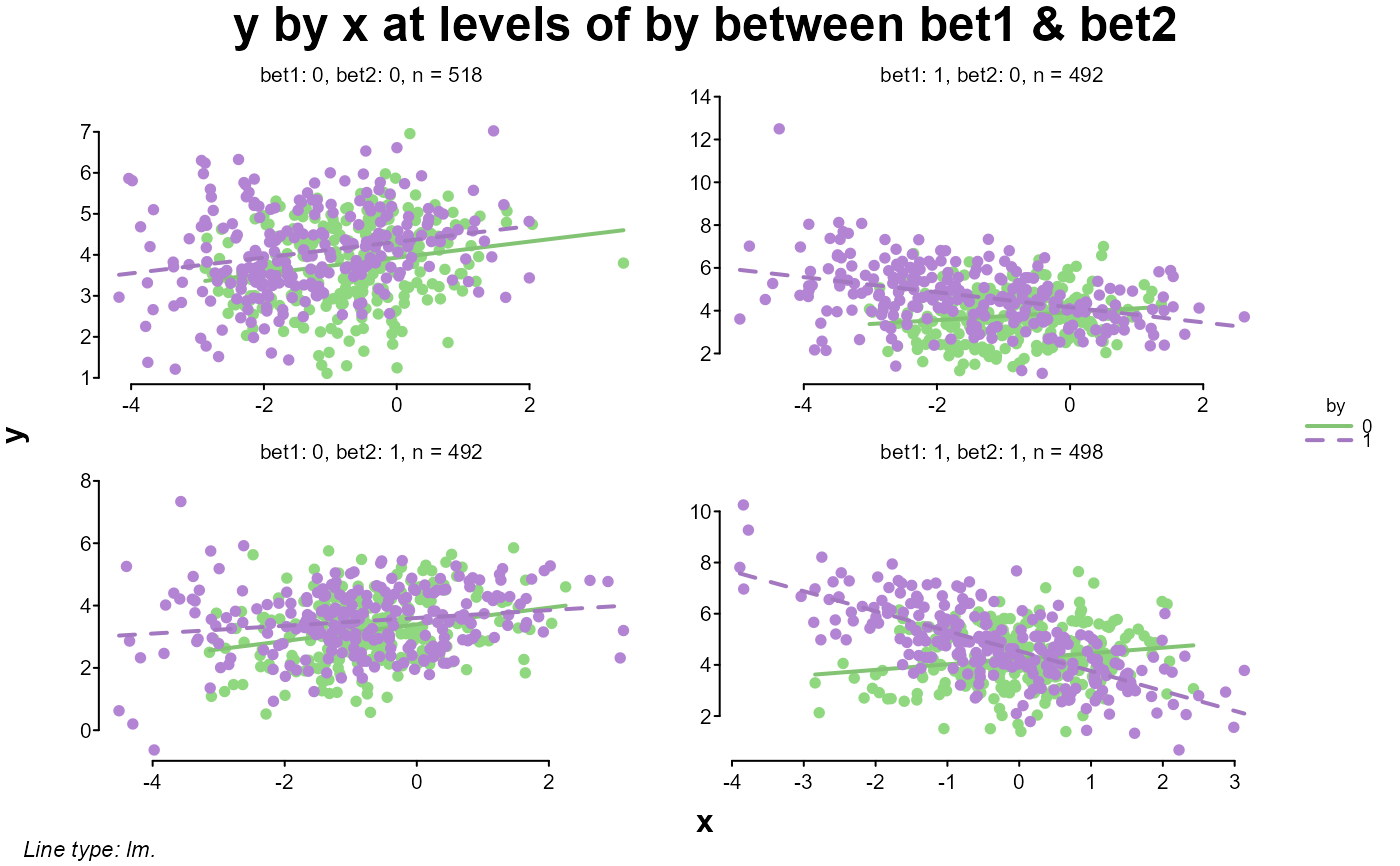# same as the last but entered by name
splot(y, x = x, by = by, between = c(bet1, bet2), data = dat)

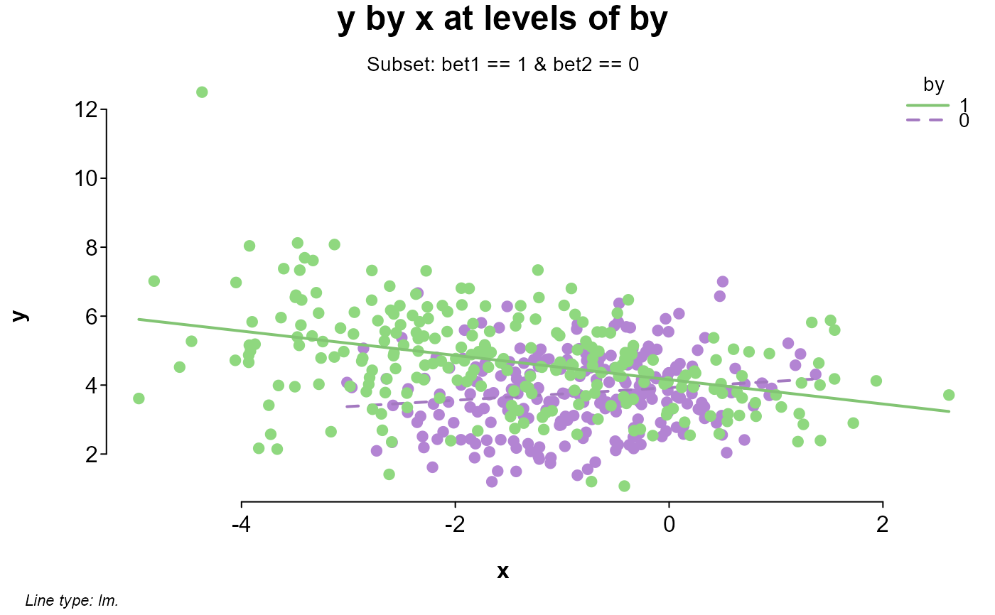
# zooming in on one of the windows
splot(y ~ x * by, dat, bet1 == 1 & bet2 == 0)


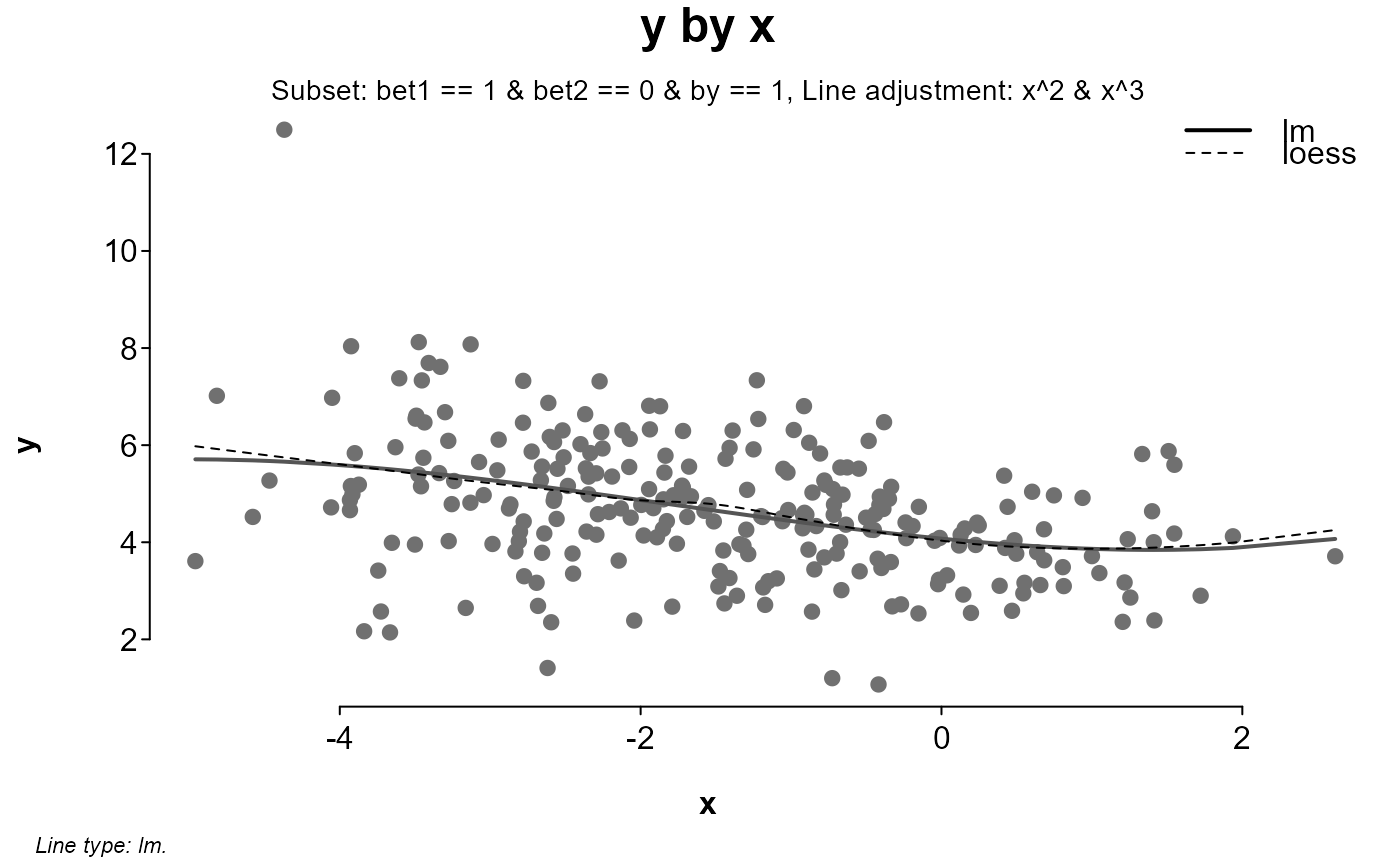
# comparing an adjusted lm prediction line with a loess line
# this could also be entered as y ~ poly(x,3)
splot(y ~ x + x^2 + x^3, dat, bet1 == 1 & bet2 == 0 & by == 1, add = {
  lines(x[order(x)], loess(y ~ x)$fitted[order(x)], lty = 2)
  legend("topright", c("lm", "loess"), lty = c(1, 2), lwd = c(2, 1), bty = "n")
})


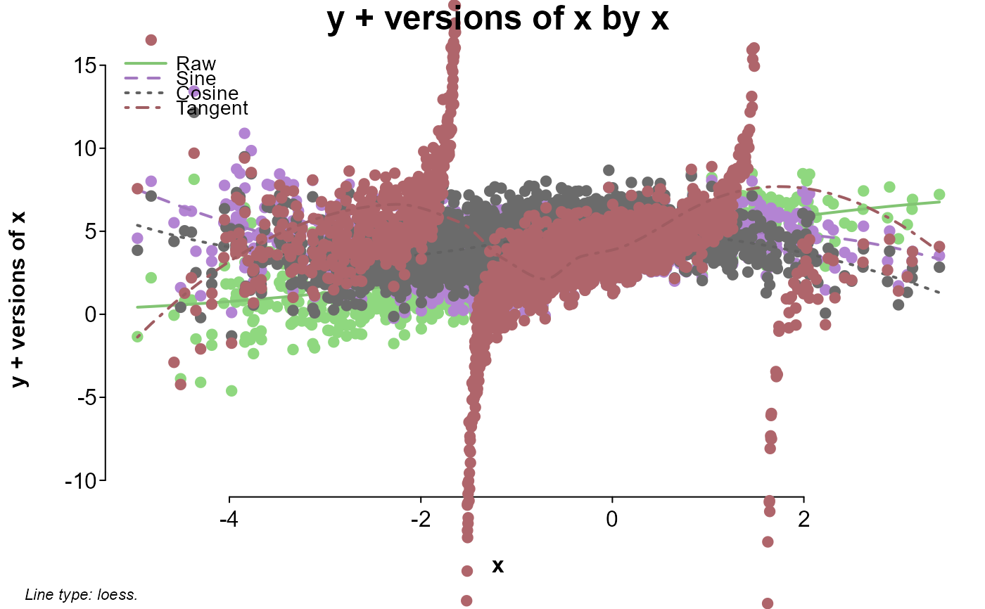
# looking at different versions of x added to y
splot(cbind(
  Raw = y + x,
  Sine = y + sin(x),
  Cosine = y + cos(x),
  Tangent = y + tan(x)
) ~ x, dat, myl = c(-10, 15), lines = "loess", laby = "y + versions of x")